View Model Results
GeoSWMM generates a wide variety of model output reports, tables and charts for showing model results. Following sections briefly demonstrate how you can view and analyze some of them after a successful model run in GeoSWMM.
View Status Report
GeoSWMM generates a summary of the overall model simulation. To view this status report:
Go to the GeoSWMM tab Results Section and expand the gallery view and from Reports section click on the Status Report (![]() ) button. It will display the status report like the following figure.
) button. It will display the status report like the following figure.
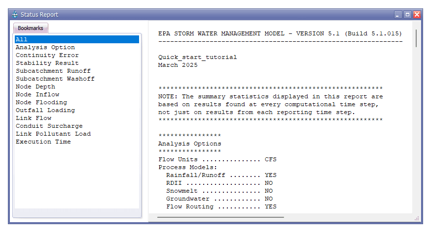
You can see the summary of simulation states at different time steps. You can browse through the results by scrolling down the cursor. Note that the extent of the status report details depends on the choice made in the Hydraulics page in Options editor.
View Time Series Plot
A time series plot graphs the values over time of specific combinations of objects and variables. Up to ten times series can be plotted on the same graph. To create a time series, plot the following needs to be done:
Go to the GeoSWMM tab Results Section and expand he gallery view and from Plots section and click on the Time Series Plot (![]() ) button. It will display a time series plot manager.
) button. It will display a time series plot manager.
On the time series plot manager, specify what time interval and what pair of objects and variables to plot. For example: specify Subcatchments as Object Category, Runoff as Variables from the dropdown list, and subcatchments S-1, S-2 and S-3 as Selected Objects. Then click View button to generate the plot. It should look like the following figure.
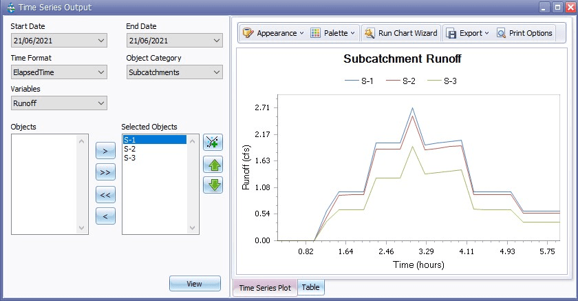
The general appearance of the chart can be defined using the Appearance option in the tool bar. Usually the ‘default’ appearance option is set and you can change it by clicking the option and choose different style from the dropdown list. Moreover, you can organize, customize and present the chart using Run Chart Wizard with a real-time preview. See in detail how to work with Run Chart Wizard.
After finishing the customization or keeping the default, you can export the chart in Pdf, Html, Mht, Rtf or Different Image formats clicking Export on the tool bar of the Time Series Plot Window. Moreover, the Printing Options button in the tool bar will allow you to edit the customized chart and print it by opening a separate window.
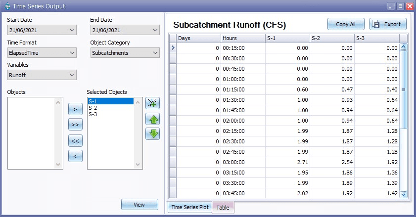
You can also extract time-based values of the specified variable for those specific objects by clicking the bottom Table tab in the Scatter Plot window and export this table by clicking the Export button on the top-right side of the window. Then you will need to browse the targeted file location in your computer to complete the process. It will look like the following figure:
View Time Series Comparison
The Time Series Comparison wizard allows the comparison between two-time series outputs of the same or different variables between the same or different objects in GeoSWMM. For example, to compare time series outputs of flow and capacity of conduit C-1 with the pressure at the pump delivery node J-1 the following needs to be done:
Go to the GeoSWMM tab Results Section and expand he gallery view and from Plots section and click on the Time Series Comparison (![]() ) Button. It will display the time series comparison wizard. Notice that there are two input columns for two analyzing variables.
) Button. It will display the time series comparison wizard. Notice that there are two input columns for two analyzing variables.
On the time series comparison manager, specify what time interval and what pair of objects and variables to plot. For example: specify Elapsed Time as Time Format, Links as Object Category, C-1 as Object in both series, and Flow and Capacity (for Series 1 and Series 2 respectively) as Variable in the wizard. Then click on the View button to generate the plot. It should look like the following figure. Notice that two vertical axes are provided for the two variables with respect to a same time axis.
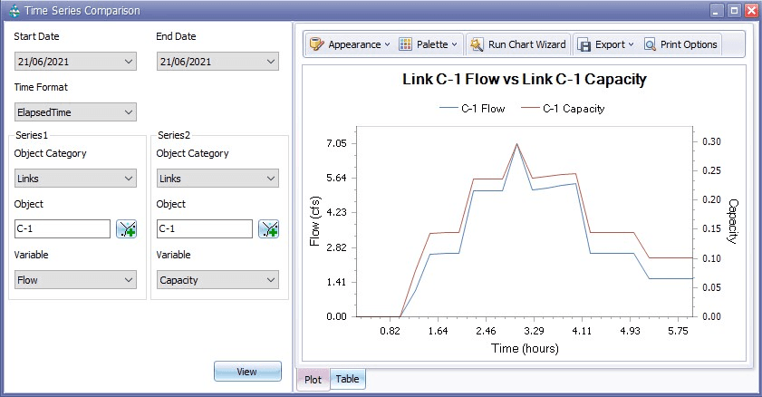
In the time series comparison window, there is a tab with Chart Appearance to edit the chart appearance and Palette, a Run Chart Wizard to customize the chart’s properties like diagram’s properties, panes, axes, point labels, chart titles, legends etc. with a real-time preview. See in detail how to work with Run Chart Wizard.
After finishing the customization or keeping the default, you can export the chart in Pdf, Html, Mht, Rtf or Different Image formats clicking Export on the tool bar of the Time Series Plot Window. Moreover, the Printing Options button in the tool bar will allow you to edit the customized chart and print it by opening a separate window.
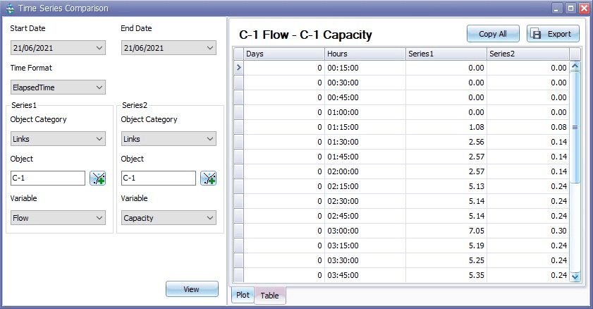
You can also extract time-based values of the specified variable for those specific objects by clicking the bottom Table tab in the Scatter Plot window and export this table by clicking the Export button on the top-right side of the window. Then you will need to browse the targeted file location in your computer to complete the process. It will look like the following figure:
View Profile Plot
The Profile Plot manager generates simulated water elevation profiles along a connected path of drainage system links and nodes at a particular point in time. For example, to create an elevation profile from junction J-4 to outfall O-1:
Go to the GeoSWMM tab Results Section and expand he gallery view and from Plots section and click on the Profile Plot (![]() ) button. The profile plot manager will open in a separate window.
) button. The profile plot manager will open in a separate window.
Specify J-4 as Start Node and O-1 as End Node in the manager. Then click on the Find Path button to see the available items in the linkage. At this stage, the profile plot manager should look like the following figure.
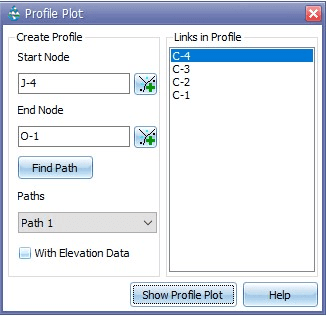
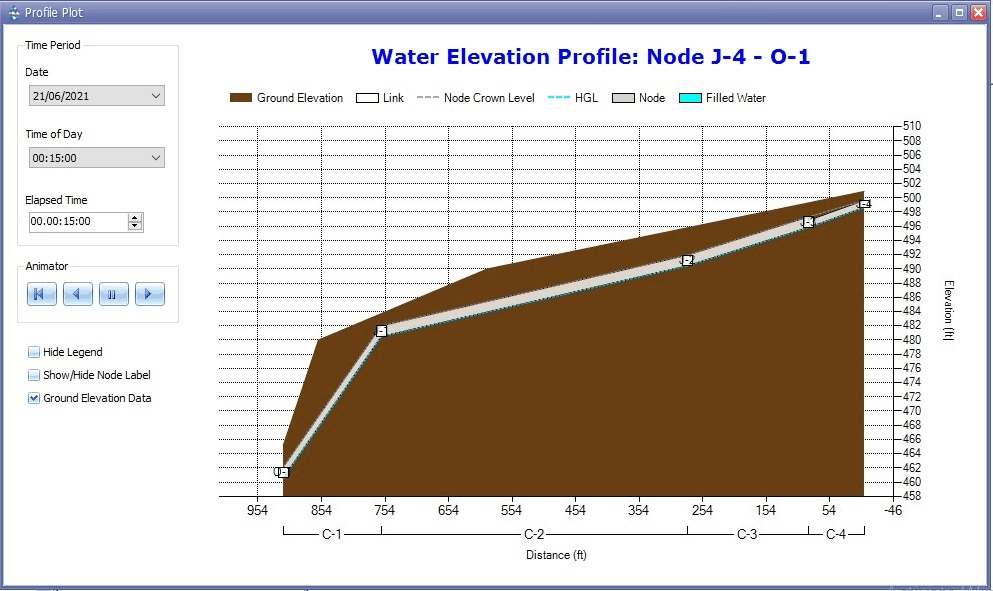
Now click on the Show Profile Plot button. The profile map from junction J-4 to outfall O-1 will be displayed like the following figure. You can animate and observe the variation of water surface level within the reporting time steps in the profile plot window.
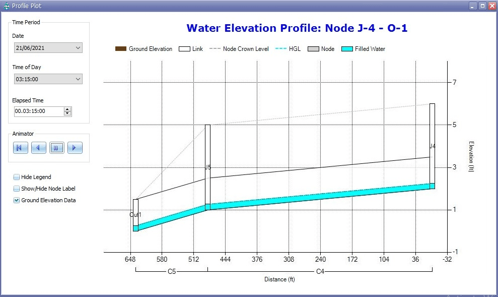
You can also perform the same plotting with the existing ground surface elevation on it. In that case you must extract the elevation of your study area from an elevation dataset (i.e. contours) by the Elevation Manager tool of GeoSWMM prior to performing with the Profile Plot manager. For more details visit at Elevation Manager.
When the extraction is done, complete the steps 1 and 2 as before. Then check the with Elevation Data option in the most bottom-left window. At this stage the window will look like the following figure.
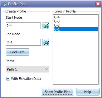
Complete the step 3 as before and the plotting window will appear like Figure 2.33.
View Output Result Table
GeoSWMM enables listing and viewing of time series output results of a single object in a table. For example, to view the tabular results for subcatchment S-1:
Go to the GeoSWMM tab Results Section and expand he gallery view and from Tables section and click Results by Object (![]() ). It will open the result table manager.
). It will open the result table manager.
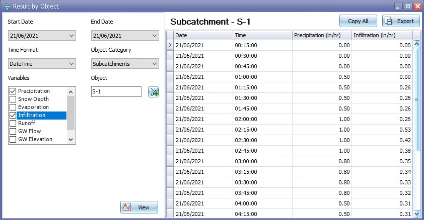
Specify Subcatchments as Object Category and S-1 as Object in the manager. Then select Precipitation and Infiltration from the variable list. Set Date Time as Time Format.
Then click on the View button to generate the table. It will appear like the following figure. You can also export the table to a spreadsheet (.csv) file from this window.
View Summary Results
The Summary Report contains tables listing summary results for each subcatchment, node and link in the drainage system. Total rainfall, total runoff, and peak runoff for each subcatchment, peak depth and hours flooded for each node, and peak flow, velocity, and depth for each conduit are just some of the outcomes included in the summary report. The Summary Results window has a dropdown list from which you select a particular topic to view as report. For this:
Go to the GeoSWMM tab Results Section and expand the gallery view and from Reports section and click on the Summary Results (![]() ) button. It will open the summary results manager. For example: specify Node Inflow as the Topic and it will look like the following figure.
) button. It will open the summary results manager. For example: specify Node Inflow as the Topic and it will look like the following figure.
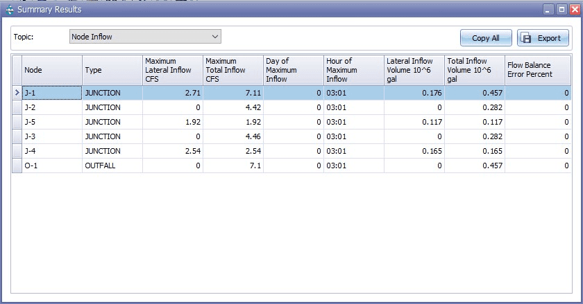
This table can be exported by clicking on the Export button on the top-right side of the window. Then browsing to the targeted file location in the computer allows to complete the process.
Export Output in CSV
GeoSWMM provides user specified result exporting option. You can choose to export result of any variable for any object in your specified format of table. To do so follow these steps:
Go to the GeoSWMM tab Results Section and expand he gallery view and from Tables section and click on the Results by variable (![]() ) button. The Export Output Window will be opened then.
) button. The Export Output Window will be opened then.
Specify Date Time as Time Format and Nodes as Object Category. Now check Depth and Total Inflow as Variables; J-1 and O-1 as Objects. At this stage the window will look like the following figure.
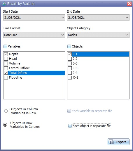
Exporting the ‘csv’ outputs in two different combinations is allowed- Objects in Column and Variables in Row and vice versa. Moreover, it is possible to export ‘Each variable in separate file’ or ‘Each object in separate file’ according to the respective combination by just checking the adjacent radio button.
Now click on the Export button. Then you will need to browse the targeted file location in your computer to complete the process. then browsing to the targeted file location in the computer will allow the user to complete the process.
View Scatter Plot
GeoSWMM allows users to select the objects and variables to be graphed against one another in a scatter plot. A scatter plot displays the relationship between a pair of variables, such as flow rate in a pipe versus water depth at a node. To create a scatter plot:
Go to the GeoSWMM tab Results Section and expand the gallery view and from Plots section and click on the (![]() ) button. The Scatter Plot Window will be opened then.
) button. The Scatter Plot Window will be opened then.
Specify what time interval and what pair of objects and variables to plot. For example: In the X- Variable list, select Subcatchments as Object Category from the dropdown list, S2 as Object and Precipitation as Variable from the dropdown list. In the Y- Variable list, select Subcatchments as Object Category from the dropdown list, S2 as Object and Runoff as Variable from the dropdown list.
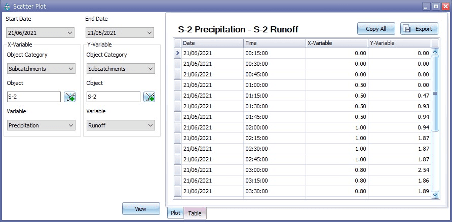
Now click on the View button. The window will look like the following figure.
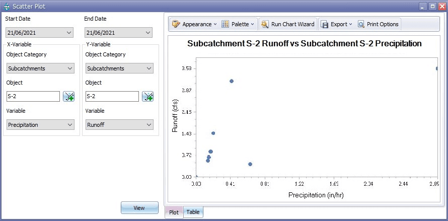
In the Scatter Plot window, there is a tab with Chart Appearance to edit the chart appearance and Palette, a Run Chart Wizard to customize the chart’s properties like diagram’s properties, panes, axes, point labels, chart titles, legends etc with a real-time preview. See Section 10.4 about working with Run Chart Wizard in detail.
After finishing the customization or keeping the default, you can export the chart in Pdf, Html, Mht, Rtf or Different Image formats clicking Export on the tool bar of the Scatter Plot Window. Moreover, the Printing Options button in the tool bar will allow you to edit the customized/default chart and print it by opening a separate window.
You can also extract time-based X-variable and Y-variable values by clicking the bottom Table tab in the Scatter Plot window and export this table by clicking the Export button on the top-right side of the window. Then you will need to browse the targeted file location in your computer to complete the process. It will look like the following figure:
